Most discovery teams validate solubility and aggregation after the biophysics screen. Moving it upstream — before SPR — gives you clean molecules, clean data, and fewer late surprises. Here is why that is now possible, and what it changes.
The old school way of doing drug discovery
Look at how a hit list usually moves through early discovery:
Hit list → biophysics screen → solubility & aggregation validation → drop, filter, retest, rework → decide
Solubility and aggregation sit near the end. They act as a checkpoint you clear once the interesting molecules have already been through the biophysics screen. On paper that looks efficient. In practice it is the most expensive place you can put them.
By the time solubility and aggregation surface, you have already spent scarce biophysics capacity — SPR time, immobilized protein, analyst hours — on molecules that should never be there in the first place. Worse, the aggregators still sitting in the hit list is a hidden risk that you have no idea when it springs up. They adsorb non-specifically onto the immobilized protein, block microfluidic channels, and foul sensor surfaces. The binding data you trusted is quietly contaminated by molecules that were misbehaving all along.
So you loop back. Retest. Rework. The one question that should have a clean answer — “is this binding real, or am I looking at an aggregator?” — stays open longer than it should.
What if you can change the order?
The modern way: put solubility and aggregation first
Now put the checkpoint at the front:
Hit list → solubility & aggregation → drop, filter, arrange → biophysics screen → decide
Profile the entire hit list up front. Drop the aggregators. Filter the poorly soluble. Arrange the survivors by how they actually behave. Then send only clean moleules into the biophysics screen. Or put the aggregators in the end, at least you know there is no false-hit because of aggregators bound to your proteins.
The difference is not cosmetic. In the old order, solubility and aggregation are a filter on survivors. In the new order, they are a filter on the whole list — which means the aggregators never reach the sensor chip, and the binding data you generate downstream is clean by construction. You stop asking whether your hits are real, because you removed the molecules that would have made you ask.
This is the shift from late surprises to early certainty. And it saves real time and money: capacity that used to be spent characterizing failures is spent advancing candidates.
What changed? Why this wasn’t possible before
Front-loading only works if you can profile the entire hit list — not just the shortlist — at the concentrations that matter, on the material you actually have and at the cost you can afford. That requires three things at once, and legacy methods give you one or the other, never all at once:
- Sensitivity below 1 µM. Binding happens at micromolar and lower, so aggregation has to be detected there too — and early, before it becomes visible turbidity. Nephelometry waits for turbidity. DLS saturates and picks up multiple-scattering artefacts. Neither catches the early onset at binding-relevant concentrations.
- Throughput to run the whole list on minimal material. HPLC-based solubility workflows has the sensitivty requirement but are roughly 100× slower and consume far more compound (~ 1 mg). Running them across a full hit list is not practical, so teams profile only the survivors — which puts us right back in the old, expensive order.
- Cost effective to run. In order for the economics to work, the cost of running solubility must be ~10x less expensive than SPR (biophysics) to warrant savings from not running compounds that aggregate. This is only possible if both throughput and compound consumption are satisfied, such that the unit economics on a compound basis is reduced.
You need all at the same time to screen the entire hit list and match the discovery timeline — That is the gap the ORYL F1 was built to close.
How the ORYL F1 profiles an entire hit list
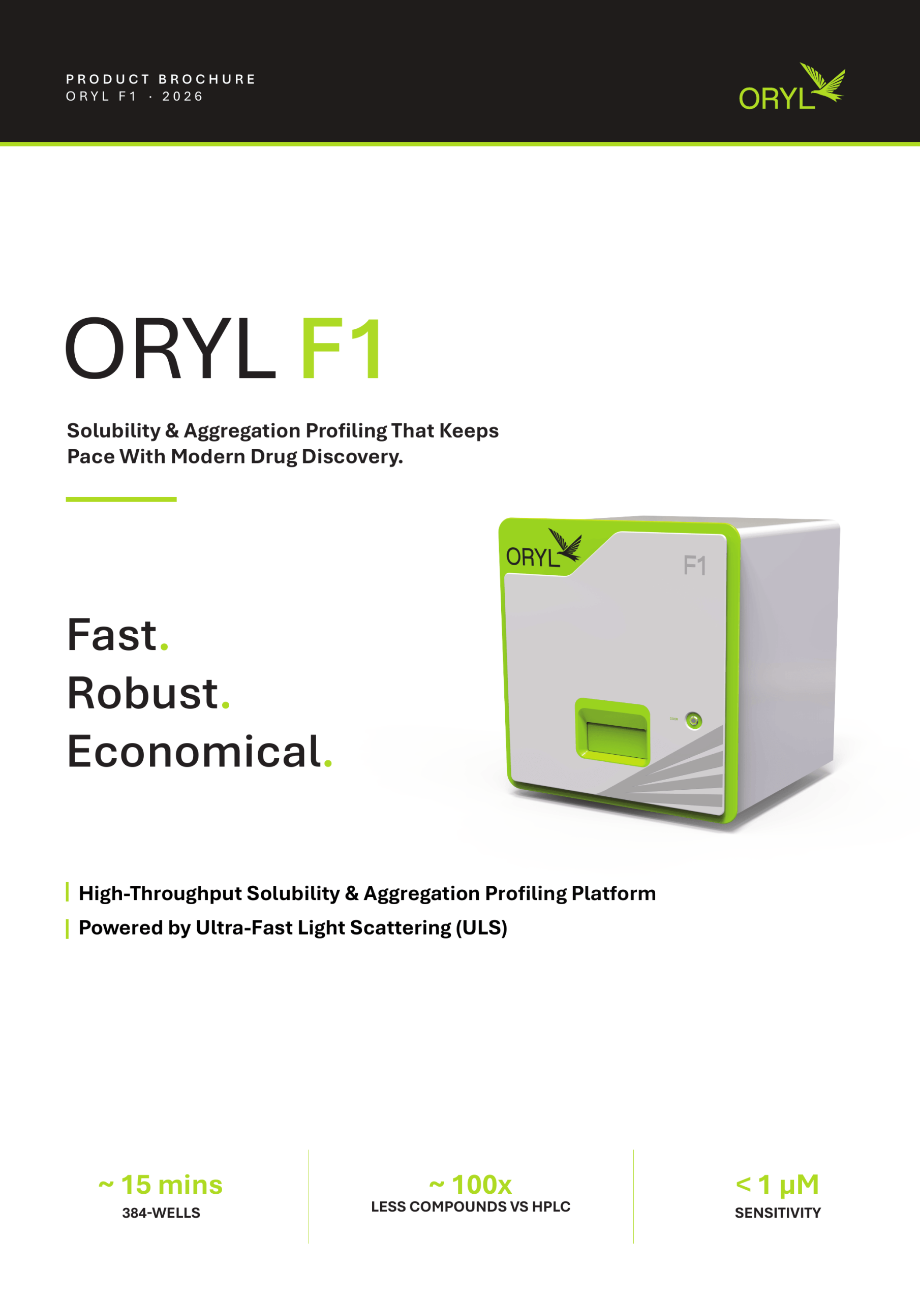
The ORYL F1 is a high-throughput, low-compound, plate-based solubility and aggregation profiling instrument, powered by Ultrafast Light Scattering (ULS). ULS combines two complementary readouts on the same sample, in a single plate-based experiment:
- Linear Light Scattering (LLS) reports particle dimension, refractive-index contrast, and how much material is present in aggregated form. Sub-µM sensitivity, and it detects the early onset of aggregation before it shows up as turbidity.
- Second Harmonic Scattering (SHS) is generated only under non-centrosymmetric molecular arrangements and is background-free in solution — so it stays informative in high-concentration biologic formulations and complex media (surfactants, micelles, bile salts) where linear light scattering methods saturate.
Read together, the two signals define the solubility limit, profile aggregation, and assign a confidence interval — including in conditions where conventional workflows fail to scale. A 384-well plate is measured in about 15 minutes, roughly 100× faster than HPLC-based solubility workflows and about 10× faster than DLS, SLS, or nephelometry. Each datapoint uses around 2 µL of a 10 mM DMSO stock. That combination — sub-µM sensitivity plus plate-based throughput at trace material — is what makes profiling an entire hit list realistic rather than aspirational.
Pre-SPR Triage spotlight
In this example, a 142-compound hit list is profiled via the ORYL F1 at SPR-relevant timepoints (1 h and 24 h), at about 15 minutes per plate.
The output is a per-compound deliverable that drops straight into the SPR operating-concentration input: for each compound, a safe-below threshold, an avoid-above threshold, a peak-amplitude readout, a timepoint-shift class, and quality flags — each with a confidence interval. Compounds sort into behavior classes that tell you exactly how to treat them:
- Canonical aggregator — misbehaves and stays that way between timepoints. Flag and drop.
- Supersaturator — soluble at 1 h, aggregating by 24 h. The kind of metastable behavior a single-timepoint read would miss entirely.
- Called at threshold but low-risk — crosses a solubility threshold but with low peak amplitude, so it can stay in the queue with eyes open.
The aggregators are flagged before they consume sensor chips and analyst time. The SPR queue that remains is clean. For a 1,000-compound campaign, ORYL puts the net savings at around $20k, with per-compound profiling more than 10× cheaper than running the molecules blind through SPR — and throughput of 1,000+ compounds profiled per day.
What it changes downstream
Reordering one step changes the character of everything after it. Your biophysics screen sees clean molecules, so it produces clean data. Your team stops spending its most expensive capacity on candidates that were destined to fail. And the decisions at the end of the funnel rest on results that were de-risked at the front, not defended after the fact.
That is the promise behind Fast, Robust, Economical: fast enough to profile the whole list, robust enough to trust the call, economical enough to do it on the material you already have. It is also modality-agnostic — small molecules, peptides, PROTACs, macrocycles, oligos, proteins, and mAbs run on the same dual-readout platform, with LLS handling small molecules and PROTACs at sub-µM sensitivity and SHS profiling biologic formulations above 50 mg/mL, where DLS and SLS saturate and HPLC stops being meaningful.
This is what modern drug discovery looks like: solubility and aggregation first, biophysics second, decisions made once — with certainty.