If we are to create a wish list for solubility measurement, what would it be? The ideal solubility measurement should be rapid, sensitive and using minimum amount of compounds. It must have a wide application coverage (different samples, solvents, pH, temperatures, excipients) and should deliver reproducible results. Preferably, the full process from sample preparation to measurement and analysis is fully automated to minimize errors and decrease hands-on time.
Is this possible? It is now. How? Using The Solvent Redistribution Method from Oryl Photonics.
Solubility measurement with the Solvent Redistribution method
The Solvent Redistribution (SR) method detects the solubility and aggregation of compounds by measuring how the solvent redistributes around the solute molecules as they transition from monomeric state to aggregated state (dimers, trimers, etc) as shown in Figure 1. The SR method detects the onset of aggregation at concentrations below the range where turbidity occurs. It is thus more sensitive than turbidity measurements while retaining the advantage of speed. Additionally, it is precise with exceptional reproducibility. Visit this page for a detailed benchmarking study.
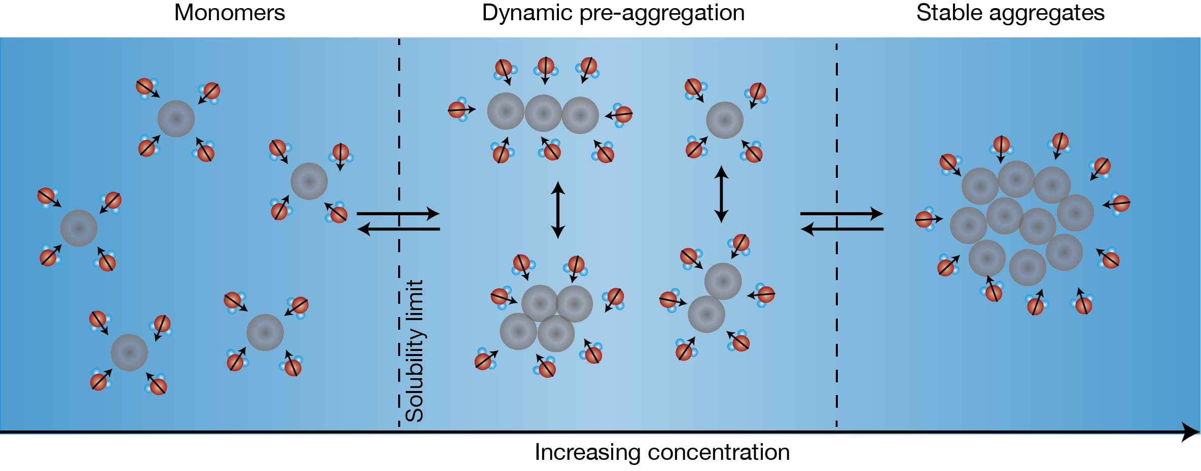
Figure 1: Schematic of aggregation for the Solvent Redistribution method. With increasing solute concentration, solute monomers transition to stable aggregates. In-between fully dissolved monomers and stable aggregates, there is a concentration range where different types of structures (dimers, trimers, etc.) co-exist. The distribution of solvent molecules around these structures change dynamically – hence the term Solvent Redistribution. Relative to the monomer state, there is an increase in the number of solvent molecules around the solute at the onset of aggregation that can be used a metric to detect the solubility limit.
Figure 1 shows the figure of concept for the SR method. With increasing concentration, the solute transitions from monomers to stable aggregates. Within the transition phase, there exists a dynamic phase of different types of structures (dimers, trimer, quadrimers, etc.) that is characterized by a higher degree of structural anisotropy. Correspondingly, the solvent around these structures redistributes and fluctuates, hence the term Solvent Redistribution. The Solvent Redistribution method is based on high-efficiency second harmonic (SH) scattering that directly measure the interfacial solvent redistributions. At the onset of aggregation (nucleation), there is an increase in the number of interfacial solvent molecules that leads to a steep increase in the SH intensity – this is used as a metric to measure the solubility limit.
Unique sensitivity
The SR method is uniquely sensitive because of:
- Wavelength separation between incoming and second harmonic beams – second harmonic photons are emitted at twice the frequency of the incoming beam (515 nm emitted, 1030 nm incoming beam) providing background-free measurements;
- Second harmonic scattering originates from the anisotropic distribution of the solvent which provides structural sensitivity and makes it selective to how substances aggregate;
- Pulsed laser that allows to synchronize the second harmonic signal with the detector.
These factors improve the signal-to-noise ratio of the SR method providing exceptionally reproducible measurements.
Minimum quantity of compounds
Since it is based on light scattering, the SR method requires minimum amount of compound and chemicals. With standard 384 well plates (or 96 half-area well plates) using 100 µL of volume, the compound requirement is typically around 2 µL of 10 mM stock solution per solubility datapoint (target maximum concentration of 100 µM). With N=3 replicates, it is now feasible to obtain solubility data per compound with ~6 µL of compound. Table 1 details the compound requirement depending on the target screen concentration (for example, if we want to qualify compounds to be soluble within a defined range of target screen concentration).
Table 1: Compound consumption with the SR Method. The compound requirement per solubility datapoint is ~4× of the target screen concentration.
| Target Screen (µM) | Volume required per solubility datapoint (µL) | Total volume required (µL) for N=3 replicates |
|---|---|---|
| 10 | 0.4 | 1.2 |
| 20 | 0.8 | 2.4 |
| 50 | 1.0 | 3.0 |
Automated and high-throughput solubility measurement
Direct transfer of stock solution

Addition of solvent
Direct screening and analysis
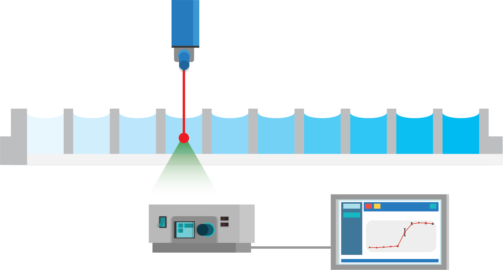
Figure 2: Fully automated solubility measurement process. The full process of solubility measurement is automated with liquid handling robots and Oryl’s SR method. In step 1, an acoustic liquid dispenser (Labcyte, Echo platform) is used to directly transfer the stock solution into well-plates with increasing concentration. In step 2, the solvent is added with peristaltic liquid dispenser (50 or 100 µL of volume). Lastly, the well-plate is measured with Oryl’s instrument. The analysis is performed automatically with Oryl’s software.
The sample preparation can be done in less than 10 minutes while a full scan of a 384 well-plate using Oryl’s instrument is done in less than 15 minutes (read time per well of 1-100 ms). Thus, it is now feasible to perform solubility screening for hundreds of thousands of compounds within a reasonable amount of time.
Reproducible and accurate solubility measurements


Figure 3: Fully automated solubility measurement with albendazole with n=3 replicates. Right plot: intensity vs concentration plot for albendazole in the concentration range 0 to 100 μM. The solid black line shows a typical linear fitting analysis that is employed in nephelometer-based measurements. Left plot: intensity vs concentration plot zooming in the concentration range 0 to 10 μM showing a steep jump in intensity, with repeatable baseline having std/mean < 1.5%. The solubility limit is calculated using a threshold of mean + 3*std of the baseline, where the baseline is defined as the average of the two lowest concentrations. Source concentration: 10 mM, final volume: 100 µL; Solvent: PBS buffer, pH 7.4; molecular weight: 265 g/mol; each well plate is measured 10× to calculate the standard deviation.
Table 2: Protocol details
| Type of measurement | Kinetic solubility (1% final DMSO concentration) |
|---|---|
| Sample preparation time | < 10 min |
| Compound requirement | typically ~2 µL |
| Read time per well | 10 ms |
| Final volume | 100 µL |
| Liquid dispensing | Echo platform for stock solution, peristaltic for solvent |
| Solvent | Standard PBS buffer (alternatives are possible: different pH, with excipients, with polymers, biologically relevant media, etc) |
Table 3: Compound consumption
| Target Conc. (µM] | Echo Transfer Vol. (nL) |
|---|---|
| 25 | 250 |
| 10 | 100 |
| 7.5 | 75 |
| 5 | 50 |
| 2.5 | 25 |
| 1 | 10 |
| 0.25 | 2.5 |
| Total (nL) | 512.5 |
Compound consumption for a target screen of 10 µM, source conc. 10 mM
Using the protocol described in Figure 2 and Table 2, we perform solubility measurement of a model compound – albendazole, 3 replicates, with a molecular weight of 265 g/mol (small molecule) in a standard 384 well-plate (Greiner, UV-star). For comparison, caffeine is used as negative control that is known to be soluble at the tested range of concentration. The results show excellent reproducibility for albendazole for each replicate. A standard nephelometry analysis by linear fitting would yield a solubility limit of ~40 µM. As the measurements have excellent reproducibility, we can zoom on the relevant concentrations (dashed red line) – right plot. The standard deviation (std) divided by the mean of the measurement is excellent at std/mean < 2%. The baseline is flat and repeatable. Thus, a straightforward analysis of solubility limit – the jump in intensity relative to the baseline by simple thresholding is feasible. The calculated solubility limit of 3.5 µM is 10× more sensitive (~40 µM) than typical nephelometric linear fitting analysis. The precision and sensitivity of the SR method eliminate the need to use higher concentrations, hence saving compounds. Table 3 shows a calculation of compound consumption for 100 µL volume for a target screen of 10 µM. Only 512.5 nL of compounds are required per solubility datapoint.
Summary
In summary, the SR method provides rapid, sensitive, efficient, and reproducible solubility measurement with minimum compound consumption. Fully automated sample preparation, measurement, and analysis open-up new avenues to perform solubility measurements at scale. It is now possible to perform hundreds of thousands of solubility measurements with excellent precision and sensitivity within a reasonable amount of time.
Applications of the SR Method
- Solubility screening of compound libraries – for fragments, small molecules.
- Solubility counter-screening – weeding-out aggregates, avoiding false positives, verifying hits.
- Solubility ‘debugging’ – investigating the effect of different excipients, different solvents, co-factors, pH, as well as solubility of excipients themselves.
Do you need to characterize the solubility of your compounds now? Oryl offers competitive and rapid Solubility Measurement as a Service (SMaaS). Download the brochure here or visit the SMaaS page.
Please contact us at smaas@orylphotonics.com for details.