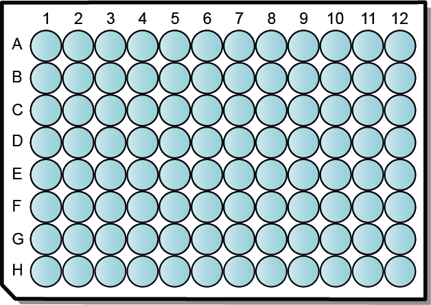
We performed solubility measurement of several poorly soluble compounds following the protocol described in figure 1. A standard 384 well-plate (Greiner 384 Well UV Star, ref. 781801) is used and the plate layout is described in figure 2. Using an acoustic liquid dispenser robot (Echo Labcyte), an increasing concentration (0, 0.1, 1, 2.5, 5, 7.5, 10, 25, 50, 75, 100 µM ) of the test compound is transferred across the 384 well-plate (dilution by row). After adding the compounds, a peristaltic liquid dispenser robot is used to transfer 100 µL of PBS buffer to each well-plate. The 384 well-plate is then directly tested in Oryl’s instruments after a 2-hour incubation period. There are 20 compounds that were tested with N=5 replicates. For comparison, the same set of compounds are tested with nephelometry. For some of the compounds, the solubility limit was measured using HPLC-UV method, with centrifugation as a pre-step to remove big aggregates and injecting the supernatant to HPLC-UV for determining the concentration of the dissolved compounds. The results are shown in Table 1.
1. Direct transfer of stock solution
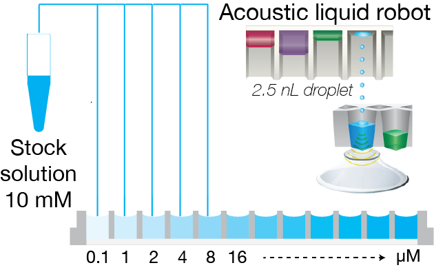
2. Addition of solvent
3. Direct screening and analysis
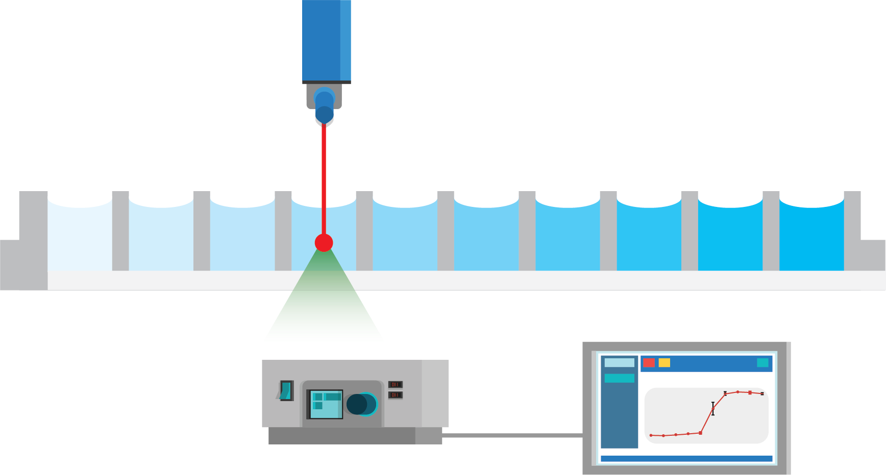
Figure 1: Protocol for fully automated solubility measurement process. The full process of solubility measurement can be automated with liquid handling robots and the Solvent Redistribution method. In step 1, an acoustic liquid dispenser (Labcyte, Echo platform) is used to directly transfer the stock solution into well-plates with increasing concentration. In step 2, the solvent is added with peristaltic liquid dispenser (100 µL of volume). Lastly, the well-plate is measured with Oryl’s instrument. The analysis is performed automatically with Oryl’s software.
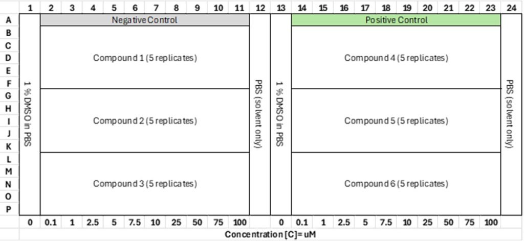
Figure 2: Experimental well-plate layout. Greiner 384 Well UV Star is used in the benchmarking study. The total volume per well is 100 µL. The solvent is PBS buffer with pH 7.4. There are 5 replicates per compound and the compound concentration is increased along each row with concentration range: 0, 0.1, 1, 2.5, 5, 7.5, 10, 25, 50, 75, 100 µM.
Table 1: Benchmarking the Solvent Redistribution method with nephelometry and HPLC-based solubility measurements. The values for Solvent Redistribution and nephelometry are measured kinetic solubility limit (in micromolar – µM) for the 20 compounds. For HPLC-based measurements, some are done in-house while the rest are taken from literature values (see superscript for reference).
| Cpd | Replicate 1 | Replicate 2 | Replicate 3 | Replicate 4 | Replicate 5 | Average Oryl | HPLC-UV | Nephelometry |
|---|---|---|---|---|---|---|---|---|
| 1 | 5.61 | 5.61 | 4.83 | 4.93 | 4.41 | 5.08 | 13.1# | 90.73 |
| 2 | 8.04 | 6.79 | 7.73 | 3.69 | 6.85 | 6.62 | 4^ | 51.78 |
| 3 | 3.34 | 3.05 | 3.27 | 3.05 | 3.76 | 3.29 | 9^ | 29.4 |
| 4 | 99.97 | 99.97 | 99.97 | 99.97 | 99.97 | 99.97* | - | >100 |
| 5 | 0.02 | 0.03 | 0.03 | 0.02 | 0.02 | 0.02 | 4.36** | 26.87 |
| 6 | 21.22 | 28.36 | 28.07 | 26.18 | 25.15 | 25.79 | 3^ | 26.55 |
| 7 | 0.20 | 0.35 | 0.33 | 1.10 | 0.84 | 0.56 | 7.5 | 38.4 |
| 8 | 7.65 | 6.79 | 7.50 | 5.56 | 5.90 | 6.68 | 7^ | 38.3 |
| 9 | 99.97 | 99.97 | 97.99 | 99.97 | 99.97 | 99.57* | - | >100 |
| 10 | 6.14 | 5.56 | 5.61 | 5.45 | 5.23 | 5.60 | 0.1 | 10.7 |
| 11 | 1.48 | 5.72 | 1.94 | 6.52 | 7.50 | 4.63 | 1 | 21.2 |
| 12 | 7.81 | 1.28 | 3.08 | 5.34 | 6.79 | 4.86 | 1 | 12.8 |
| 13 | 5.28 | 5.03 | 3.92 | 4.50 | 3.84 | 4.51 | 2.5^ | 7.71 |
| 14 | 99.97 | 99.97 | 99.97 | 99.97 | 99.97 | 99.97* | - | > 100 |
| 15 | 16.52 | 7.42 | 8.98 | 5.23 | 5.56 | 8.74 | 12.7# | 22.40 |
| 16 | 0.70 | 0.10 | 0.26 | 0.26 | 1.16 | 0.50 | - | 7.85 |
| 17 | 7.81 | 6.52 | 6.65 | 7.81 | 5.72 | 6.90 | 2^ | 51.02 |
| 18 | 15.10 | 17.20 | 13.53 | 16.36 | 19.59 | 16.36 | 1 | 21.7 |
| 19 | 1.50 | 1.79 | 3.44 | 2.68 | 2.87 | 2.46 | 19.1# | 7.11 |
| 20 | 0.01 | 0.14 | 0.09 | 2.35 | 0.01 | 0.52 | 0.1 | 17.5 |
# Advanced Drug Delivery Reviews 59 (2007) 546-567, pH 6.5 in 50 mM phosphate buffer
^ Anal. Chem. 2009, 81, 3165–3172, pH 7.4, HEPES buffer
** Assay Drug Dev. Technol. 2007, vol 5, no. 4

Figure 3: Summary of the measured solubility values for 20 compounds by directly comparing the Solvent Redistribution method, nephelometry and HPLC-UV based measurements.
Figure 3 shows that the Solvent Redistribution method is comparable in terms of sensitivity to HPLC-UV method, with both methods more sensitive than nephelometry. In table 3, some of the values for HPLC-UV are obtained from literature (see superscript). It should be noted that these values should be taken carefully as there is a huge spread in the variability of solubility values in literature (see Perspectives in solubility measurement and interpretation doi: 10.5599/admet.686).
Results
Table 1 and figure 3 clearly shows that The Solvent Redistribution method produces sensitive and reproducible measurements. Although 5 replicates were used in this study, the results show reproducible measurements that 3 replicates are more than sufficient. Figures 4-6 show some selected solubility plots that demonstrate its sensitivity and accuracy. The key feature of the Solvent Redistribution method is the repeatable baseline measurements with std/mean < 5%. With this precision, it is straightforward to detect the jump in intensity that corresponds to the solubility limit and allows for automated solubility analysis. We define a threshold as mean + 3*standard deviation of the baseline, with the baseline defined as average intensity of the 2 lowest concentrations. The solubility limit is calculated as the concentration at which the threshold is reached (see figure 4).
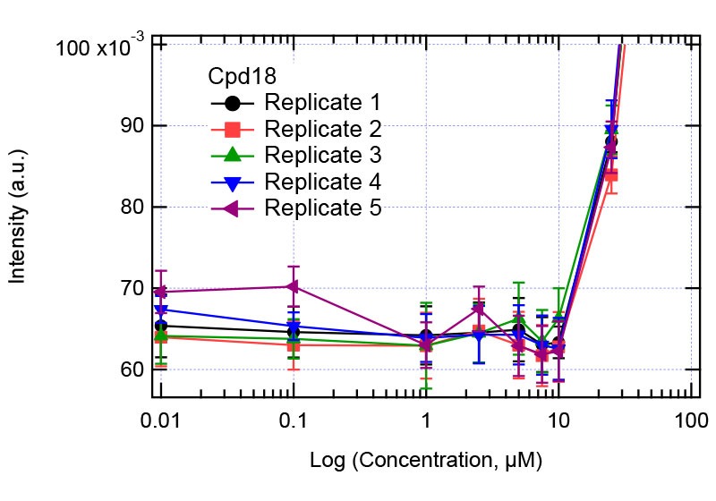

Figure 4: Solubility analysis plot for Compound 18. Right plot: full concentration range. Left plot zooms in the concentration range 1-10 µM showing the jump in intensity.
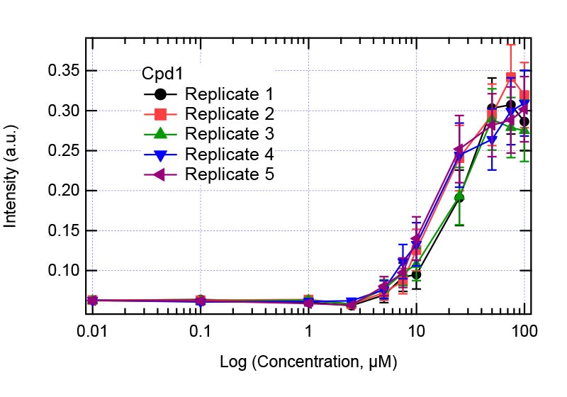
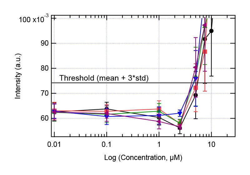
Figure 5: Solubility analysis plot for Compound 1. Right plot: full concentration range. Left plot zooms in the concentration range 1-10 µM showing the jump in intensity.
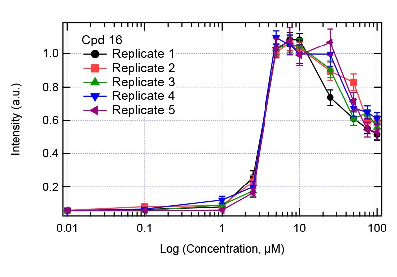
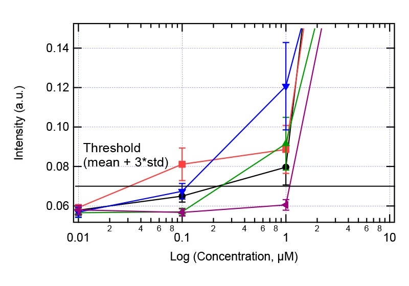
Figure 6: Solubility analysis plot for Compound 16.Right plot: full concentration range. Left plot zooms in the concentration range 1-10 µM showing the jump in intensity.
Conclusion
The Solvent Redistribution method is able to detect the solubility limit of drug-like compounds (mostly small molecules) providing results that are comparable to HPLC-UV and more sensitive than nephelometry. The full solubility measurement process is automated: from sample preparation using acoustic robot and peristaltic liquid dispenser to direct screening and analysis with Oryl’s instrument. The Solvent Redistribution method provides high-throughput and reproducible measurements with excellent sensitivity (<1 µM, small molecules). Combined with minimum use of compounds, the Solvent Redistribution method opens-up new avenues to perform solubility measurements at scale. Example applications are characterization of compound libraries, hit validation in early state drug discovery to solubility debugging with different solvents, pH and excipient combinations.
Acknowledgements
All the experiments presented in this benchmarking was done in collaboration with the Biomolecular Screening Facility (BSF) at EPFL. We express our gratitude to the BSF team, specifically Antoine Gibelin, Jonathan Vesin, Marc Chambon and Prof. Gerardo Turcatti.